Linear Curve Fits
INTRODUCTION
After taking measurements in the presence of noise or other inaccuracies, we often want to find a function which best matches or predicts that data. In mathematics, the exercise of adjusting parameters in some predicting function for this purpose is called “curve-fitting” or “regression.”
If we draw a straight line through the measured data points, that function is obviously “linear.” But in a more general sense regression is said to be “linear” if multiplying the parameters by some constant, “c”, increases the total value of the function by that same constant factor. For a single variable “x” and one constant, this means
![]()
In all such cases there is a unique solution for the parameter set. That is to say for an independent variable “y” that is caused by or “determined” by the dependent variable “x”, we have “n” simultaneous measurements of both variables as
![]()
We then want to determine the unique set of “m+1” parameters

that when used in an expansion of a family of functions ![]()

will minimize the total squared error between the measurements and functional predictions as

The functions ![]() are typically a set of
orthogonal functions but could simply be a polynomial power series where
are typically a set of
orthogonal functions but could simply be a polynomial power series where
![]()
or

LEAST SQUARES CURVE FIT
We start by taking the derivatives of the squared error with respect to the each one of the “m+1” parameters as follows

or by rearranging terms, we have

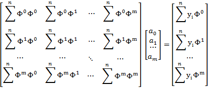
These “m+1” equations can then be more concisely expressed in a matrix format as follows

which allows for a direct calculation of the parameters using perhaps the Gauss-Jordan method.
LINEAR LEAST-SQUARES FIT
For a linear polynomial or straight line with m=1, then
![]()
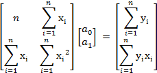
and the matrix is

This can be directly solved as


QUADRATIC LEAST-SQUARES FIT
For a quadratic polynomial with m=2, then
![]()
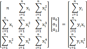
and the matrix is

But if we rewrite the matrix as

then the exact solution is
![]()
![]()
![]()
![]()
LEGENDRE LEAST-SQUARES FIT
The first few Legendre polynomials are
![]()
![]()
![]()
![]()
![]()
And the Legendre polynomials satisfy the recurrence relation
![]()
or more directly
